Here’s a demonstration that you should do integrated, or Bayesian, power analysis when making power calculations. Consider the case when, to the best of your knowledge, the true effect size is distributed according to the gamma distribution with parameters \(2\) and \(2\). You know the standard deviation is 1, to keep things simple.
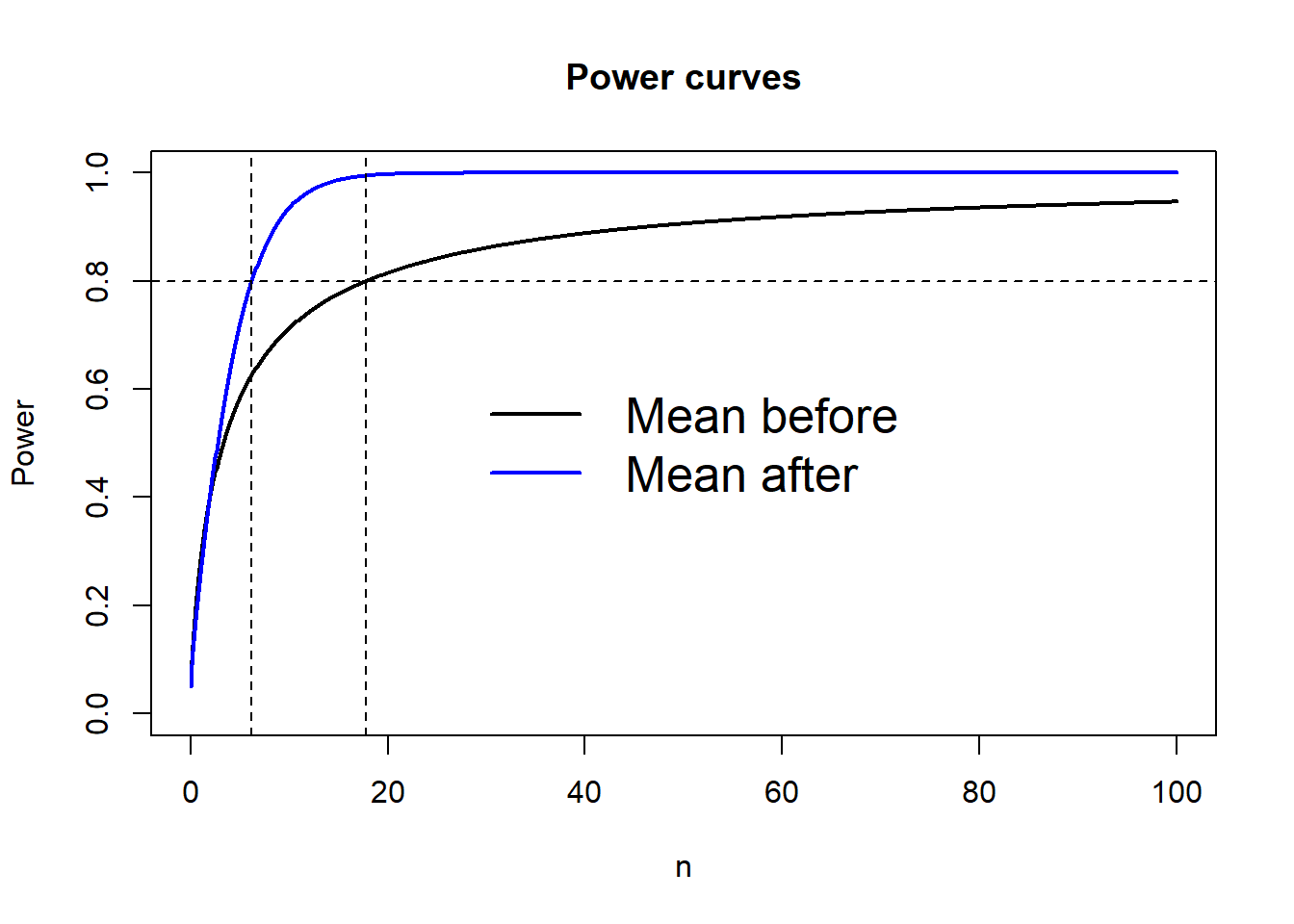
In this case, taking the mean of the effect size distribution (1) and do power analysis on that would be a mistake. Instead, you should integrate the power with respect to the distribution and solve it for \(n\). In this particular case, you want a power of \(0.8\), the difference is striking – \(n = 7\) for the incorrect approach and \(18\) for the correct approach.
To see why, define the power of the Z-test with gamma distributed effect size here:
mu = seq(0.01, 3, by = 0.01)
d = \(x) dgamma(x, 2, 2)
f = Vectorize(\(n) integrate(\(x) pnorm(qnorm(0.95) - x * sqrt(n)) * d(x), 0, Inf)$value)
The desired sample sizes can be computed as follows.
mean_after = optimize(\(n) (f(n)-0.2)^2, c(1, 30))$minimum
mean_before = (qnorm(0.95) - qnorm(0.2))^2
c(mean_after, mean_before)
## [1] 17.761238 6.182557In a plot, we get:
n = seq(0, 100, by = 0.1)
plot(n, 1 - f(n), ylim = c(0, 1), type = "l", lwd = 2, main = "Power curves", ylab = "Power")
lines(n, 1 - pnorm(qnorm(0.95) - sqrt(n)), lwd = 2, col = "blue")
legend("center", legend = c("Mean before", "Mean after"), col = c("black", "blue"), lwd = 2, bty = "n", cex = 1.6)
abline(v = mean_after, lty = 2)
abline(v = mean_before, lty = 2)
abline(h = 0.8, lty = 2)