This post is about counterfactuals in the probit model. I wrote this while reading Pearl et al’s 2016 book Causal Inference in Statistics: A Primer.
The probit model with one normally distributed covariate can be written like this:
\[ \begin{eqnarray*} \epsilon & \sim & N\left(0,1\right)\\ X & \sim & N\left(0,1\right)\\ Y\mid X,\epsilon & = & 1_{X+\epsilon\geq0} \end{eqnarray*} \]
Now we wish to find the density of the counterfactual \(Y_{x}\), see Pearl et al. (2016) for definitions. The density of \(\epsilon\) given \(X=x\) and \(Y=1\) is
\[ \begin{eqnarray*} p\left(\epsilon\mid X=x,Y=1\right) & = & \frac{p\left(x=x,Y=1\mid\epsilon\right)p\left(\epsilon\right)}{p\left(x=x,Y=1\right)}\\ & = & \frac{p\left(Y=1\mid\epsilon,x=x\right)p\left(x=x\right)p\left(\epsilon\right)}{p\left(x=x,Y=1\right)}\\ & \propto & 1_{x+\epsilon\geq0}p\left(x=x\right)p\left(\epsilon\right) \end{eqnarray*} \] or the normal density truncated to \(\left[-x,\infty\right)\), or \(\phi_{\left[-x,\infty\right)}\left(\epsilon\right)\).
Probability of Necessity
Now we’ll take a look at the probability of necessity. The most obvious way to generalize the probability of necessity to continuous distributions is to allow the counterfactual \(x'\) to be a parameter of the counterfactual \(Y_{x'}\), like this:
\[ \begin{eqnarray*} P\left(Y_{x'}=0\mid X=x,Y=1\right) & = & 1-\int_{-x}^{\infty}1_{x'+\epsilon\geq0}\phi_{\left[-x,\infty\right)}\left(\epsilon\right)\\ & = & 1-\int_{\max\left\{ -x,-x'\right\} }^{\infty}\phi_{\left[-x,\infty\right)}\left(\epsilon\right)d\epsilon\\ & = & 1-\frac{\min\left(\Phi\left(x\right),\Phi\left(x'\right)\right)}{\Phi\left(x\right)} \end{eqnarray*} \] Let’s plot this function.
x <- seq(-3, 3, by = 0.01)
x_hat <- 0

ps <- function(x, x_hat) 1 - pmin(pnorm(x_hat), pnorm(x))/pnorm(x_hat)

plot(x = x, y = ps(x, x_hat),
     type = "l",
     xlab = "Counterfactual x'",
     ylab = "Probability",
     main = "Counterfactual Probabilities, x = 0")
grid()
lines(x = x, y = ps(x, x_hat), type = "l")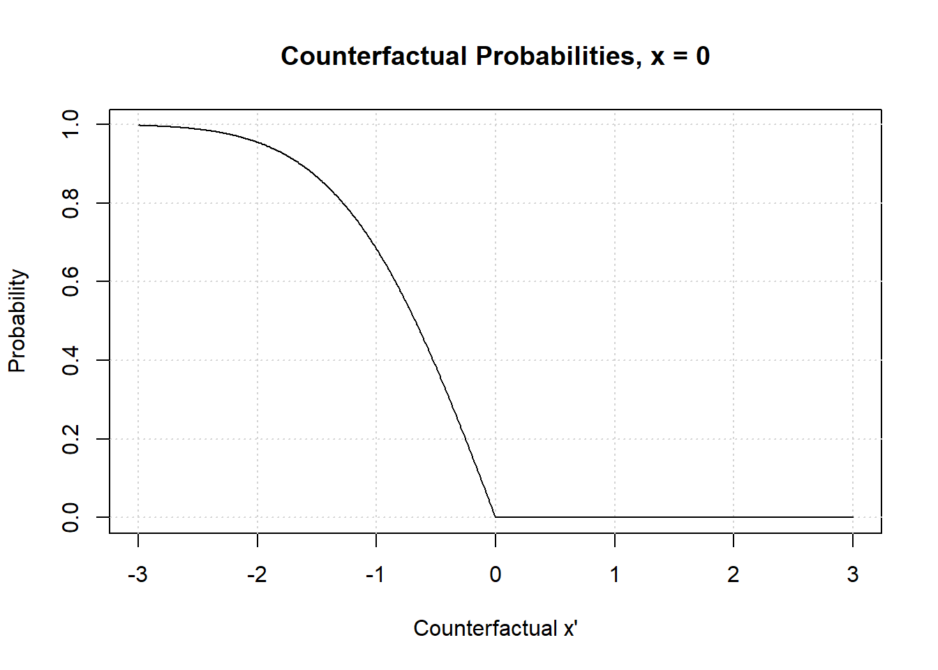
There is nothing too strange. The probability of necessity goes to \(0\) as \(x\to-\infty\), which is what you would expect. For the probability of \(Y=1\) becomes really slim as \(x\to-\infty\). When \(x'>0\) the probability of necessity is \(0\), as you will always observe \(Y=1\) counterfactually when \(X=x'\) if you observed \(Y=1\) with \(X=x!\)
Integrated Probability of Necessity
A more complicated question is: What rôle did the fact that \(X=x\) have in \(Y=1\)? Or, if \(X\) wasn’t \(x\), what would \(Y\) have been? With some abuse of notation, \(P\left(Y_{X'}=0\mid X=x,Y=1\right)\) answers this question, where \(X'\) is an independent copy of \(X\).
\[ \begin{eqnarray*} P\left(Y_{X'}=0\mid X=x,Y=1\right) & = & 1-\int_{-\infty}^{\infty}\int_{\max\left\{ -x,-x'\right\} }^{\infty}\phi_{\left[-x,\infty\right)}\left(\epsilon\right)\phi\left(x'\right)dx\\ & = & 1-\int\frac{\min\left(\Phi\left(x\right),\Phi\left(x'\right)\right)}{\Phi\left(x\right)}\phi\left(x'\right)dx\\ & = & 1-\int_{x}^{\infty}\phi\left(x'\right)dx-\frac{1}{\Phi\left(x\right)}\int_{-\infty}^{x}\Phi\left(x'\right)\phi\left(x'\right)dx\\ & = & 1-\Phi\left(-x\right)-\frac{1}{2}\frac{1}{\Phi\left(x\right)}\left[\Phi\left(x\right)-\Phi\left(x\right)\Phi\left(-x\right)\right]\\ & = & \frac{1}{2}\Phi\left(x\right) \end{eqnarray*} \]
Now let’s plot this.
counter = function(x) 0.5*pnorm(x)

plot(x = x,
     y = counter(x),
     type = "l",
     xlab = "Actual x",
     ylab = "Probability",
     main = "Counterfactual Probabilities")
grid()
lines(x = x,
     y = counter(x),
     type = "l")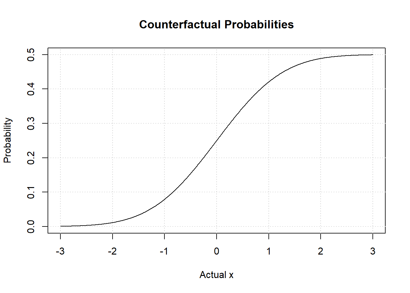
Notice the asymptote at \(0.5\). No matter how large \(X=x\) we observe together with \(Y=1\), we can never be more than \(0.5\) certain that \(Y=0\) if we were to draw an \(x\) once again. The asymptote at \(0\) if we had observed at very small value \(X=x\) together with \(Y=1\), and we were to draw again, we would be really certain that \(Y=1\) would happen once again.